“The power of a statistical test is the probability that it will yield statistically significant results. Since statistical significance is so earnestly sought and devoutly wished for by behavioral scientists, one would think that the a priori probability of its accomplishment would be routinely determined and well understood. Quite surprisingly, this is not the case. Instead, if we take as evidence the research literature, we find evidence that statistical power is frequently not understood and, in reports of research where it is clearly relevant, the issue is not addressed.” Cohen, 1988, p. 1.
Sufficiently powered studies are of utmost importance for the field of Communication Science (or any other discipline obviously). Only with sufficiently large sample sizes, we are able to detect the effects we are interested (usually rather small) with a appropriately low false negative rate. Unfortunately, there is evidence that many subfields in Communication Science are suffering from underpowered studies (see e.g., Lanier et al., 2019; Elson & Przybylski, 2017). As I am often asked about what power actually is and how to conduct power analysis, the following blogpost aims to introduce the concept of power and provide guidelines for how to incorporate power analyses as a standard practice in confirmatory research. It is my hope that it can work as a starting point for engaging with this topic more deeply.
I will first introduce the concept of statistical power in an a fictional example based on simulated data. I then define power more formally and introduce factors that affect power. I then introduce the concept of “power analysis” more broadly. At the core of this post, I show how one can conduct “simple” power analysis in R (using the package pwr and simulations; obviously power analyses can become quite complex, a while ago e.g., I wrote a blogpost about simulating power for SEMs, which is more difficult and requires more assumptions. ). Finally, I outline some guidelines and provide examples for how to report power analyses in academic work.
A simple example (using simulations)
Power can best be understood through an example. Let’s imagine that we are interested in testing whether people perceive a stronger norm to disclose themselves on social media, when the majority of other users disclose themselves (cf. the study by Masur, DiFranzo & Bazarova, 2021). In this experiment, participants are exposed to a social media feed that varies with regard to how many of the users disclosed themselves visually (5% vs. 80%). Afterwards, we measure norm perceptions. The assumption is that the more people disclose themselves, the higher the perceived norm.
Just because we can, we will simulate the true effect in the population from which the draw our sample in the experiment:
# Load package
library(tidyverse)
# Set seed to ensure reproducibility
set.seed(5)
# Simulate true effect in the population
n <- 1e5
control <- rnorm(n, 4, 1)
treatment <- rnorm(n, 5, 1)
pop <- tibble(condition = rep(c("control", "treatment"), each = n),
outcome = c(control, treatment))
head(pop)## # A tibble: 6 × 2
## condition outcome
## <chr> <dbl>
## 1 control 3.16
## 2 control 5.38
## 3 control 2.74
## 4 control 4.07
## 5 control 5.71
## 6 control 3.40This data set now represent the population from which we draw and how they would react to the different stimuli. Let’s quickly plot the distributions to get a better feel for the strength effect.
p1 <- ggplot(pop, aes(x = outcome, fill = condition)) +
  geom_density(alpha = .3) +
  theme_void() +
  theme(legend.position = "bottom")
p1
We can see that two distributions overlap considerably, but the central tendencies clearly suggest a difference. Now, let’s conduct our experiment. We sample n = 10 people from this population, which are by
definition randomly either in the control or in the treatment condition.
set.seed(11)
exp <- sample_n(pop, size = 10)
head(exp)
## # A tibble: 6 × 2
## condition outcome
## <chr> <dbl>
## 1 control 4.10
## 2 treatment 4.76
## 3 control 3.82
## 4 control 6.62
## 5 control 3.09
## 6 treatment 2.92Let’s see how these 10 people map onto the true population. We can do so by plotting them as points on the x-axis.
p1 +
  geom_point(aes(x = outcome, y = 0, fill = condition),
             data = exp, alpha = .8, shape = 21, size = 5, color = "black")
It seems we got a bit unlucky. The difference that is clearly visible in the population is not as apparent in the sample. Let’s confirm our suspicion and actually test the difference using a standard t-test:
t.test(outcome ~ condition, exp)##
## Welch Two Sample t-test
##
## data: outcome by condition
## t = -0.81441, df = 5.688, p-value = 0.4482
## alternative hypothesis: true difference in means between group control and group treatment is not equal to 0
## 95 percent confidence interval:
## -3.225805 1.630822
## sample estimates:
## mean in group control mean in group treatment
## 3.994465 4.791956Indeed, the difference is not significant, even though we know that the effect does exist in the population. So what went wrong? Well, the study was underpowered. In other words, the sample size was too small to have a sufficiently high change to detect the effect.
So what would happen if we sample more people (e.g., n = 100)?
set.seed(11)
exp2 <- sample_n(pop, size = 100)

p1 +
  geom_point(aes(x = outcome, y = 0, fill = condition),
             data = exp2, alpha = .8, shape = 21, size = 5, color = "black")
Now, it seems that the two groups (shown as circles in the figure above) are more “in line” with the distribution of the population. Let’s again test the mean difference and voila, the difference now is significant.
t.test(outcome ~ condition, exp2)##
## Welch Two Sample t-test
##
## data: outcome by condition
## t = -4.67, df = 91.213, p-value = 1.033e-05
## alternative hypothesis: true difference in means between group control and group treatment is not equal to 0
## 95 percent confidence interval:
## -1.3850141 -0.5584102
## sample estimates:
## mean in group control mean in group treatment
## 4.047700 5.019412What we can learn from this example is the following: The probability of finding a significant effect based on our sample (given that the effect actually exist) is contingent on several aspects:
- the size of our sample (n1 =10, n2 = 100)
- the strength of the true effect
- the significance level (if we would have chosen a stricter level, such as e.g., 1%, the probability of finding a significant effect would be lower)
- the type of analysis the we are conducting (in this case a t-test)
And the probability of finding a significant effect given these parameters is what we are going to talk about in this chapter: it is what we call statistical power!
What is power?
The concept “statistical power” refers to the probability of correctly rejecting a null hypothesis (H0) when the
alternative hypothesis (H1) is true. It can be formally written as 1-beta, and represents the chances of a true positive detection conditional on the actual existence of an effect to detect. As the power of a test increases, the probability of making a type II error, which means wrongly failing to reject the null hypothesis decreases (false negative result). In simpler words, the more power we have, the less likely we are to assume that there is no effect, even though the effect actually exists (see Figure 1).

Power is determined by several factors that are often contingent on the exact study that is conducted. But in any case, it is primarily determined by three factors:
—
- The effect size
- The significance level
- The sample size
—
The effect size can be a direct value of the quantity of interest (e.g, b) in a regression analysis or the mean difference in a t-test), but it can also be a standardized measure that also accounts for the variability in the population (e.g., beta) in regression analysis or Cohen’s d in a t-test). In a power analysis (see further below), this parameter is oft utmost interest. Before we collect data, we can only guess the magnitude of the effect. At times, we might have information from prior research that informs our estimation. But even if no similar study exists, we can make informed guesses. For example, Rain, Levine & Weber (2018) found an average effect size of r = .21 across 149 meta-analyses spanning 60 years of communication research. This could be a useful baseline for a power analysis (if one can reasonably assume that one’s own study is not different than the average communication science study!). Another alternative would be to consider the smallest effect size that one would still consider sufficient support for the hypothesis under investigation. For example, Purington et al. (2021) investigate the impact of a experiential learning platform on subsequent knowledge increase as assessed in a 8-item knowledge test. They argued that the smallest (unstandardized) effect size that would still speak for the effectiveness of the platform corresponds to participants who received the intervention having 1 more correct answer in the test compared to this who did not receive the intervention. The concept of the smallest effect size of interest (SESOI) can also be applied more generally. For a given hypothesis, what would be the smallest standardized effect size that still supports the hypothesis? Often, we may then resort to an effect size of e.g., r = |.10|, which represents a “small” effect according to Cohen (1988).
The significance level refers to the false positive rate and is usually set to 5%. One way to increase the power of a hypothesis test would be to use a larger significance level (e.g., 10%). This increases the chance of rejecting the null hypothesis (obtaining a statistically significant result) when the null hypothesis is false; that is, the effect actually exists. But, at the same time, it heightens the risk of obtaining a statistically significant result when the null
hypothesis is not false; that is, the effect does not actually exist. Thus, although a less conservative significance level may increase power to detect a statistically significant result when the effect is true (lower false negative rate), it heightens the probability of obtaining a statistically significant effect when the effect does not exist (higher false positive rate).
The sample size greatly determines power as it affects the sampling error inherent in a test. The larger the sample size, the more it resembles the population from which it was drawn. If all other factors are kept equal, effects are generally harder to detect in smaller samples. Thus increasing the sample size is often the easiest way to boost the statistical power of a test.
Given the entanglement of these factors with power, we can compute each of them based on all others. So if the effect size, the sample size, and the significance level is known, we can compute the power. And
vice versa, if we know the effect size, the significance level and the power, we can compute the necessary sample size. This is used in the so-called “power analysis”, which we discuss in the next section.
Before we do so, however, we have to note that next to these three pivotal factors, there are also other aspects influencing the power of a hypothesis test. For example, measurement precision also affects power. The better or measures (i.e., higher reliability), the higher the power. Another influential factor is the design of the study and what analysis is used (see further below).
Power analysis
A power analysis most often refers to calculating the minimum sample size required to detect an effect of a certain magnitude given a certain significance level and power goal. For example, before I collect my data, I would like to know how many participants I should recruit. Given the norm of the field, I set the significance level to 5%. I further have heard that I should test my effect with an equally strict power, so I set the power to 95%. Based on prior research, I assume that the effect size of interest should be r = .10. The type of analysis is a correlation analysis. So, I know all three important factors as well as the type of analysis. How can I compute the necessary sample size? The formula for calculating the necessary sample size for a correlation test is:
where n is the sample size, Z~1-alpha/2~ is the z-score corresponding to the desired level of significance, Z1-beta is the z-score corresponding to the desired power of the test, and r is the expected magnitude of the correlation between the two variables. For our example, it can thus be computed like so:
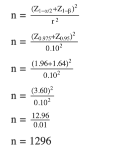
This means that the study will need to have a sample size of at least 1,296 in order to have a power of 95%, a significance level of 5%, and an effect size of r = 0.10. As mentioned earlier, this is just an approximation, and the actual sample size needed may vary depending on the specific characteristics of the study.
However, it has to be noted that the example above is what we would call an “a priori power analysis”. The term “power analysis” is broader and refers to at least three types of analyses that differ with regard to when they are usually conducted and their respective goals (see Table below).
| Type of analysis | Definition | What is estimated? |
|---|---|---|
| A priori power analysis | An analysis that is usually computed before the data is collected to estimate the necessary sample size that allows to test a certain effect with sufficient power given the level of significance | The sample size (n) |
| Post-hoc sensitivity analysis | An analysis that is usually conducted after the data collection to find out what effect size can still be tested with sufficient power given the significance level and the size of collected data set | The effect size (e.g., r, beta coefficient or Cohen’s d) |
| Post-hoc power analysis | An analysis, usually after the data collection, to find out what power was achieved given the collected sample, the significance level and the found effect size | Power (1-beta-error) |
Power analysis in R
There are different ways to compute power (or rather the necessay sample size) in R. Very broadly speaking, we can differentiate between calculating power (e.g., with packages such as pwr) or by simulating power (e.g., with packages such as MonteCarlo. In the following, I will exemplify both approaches.
Power Calculations
For simple analyses, we can often solve the above described challenge of computing the necessary sample size mathematically. In R, we have the package pwr, which provides various functions that can be used for both sensitivity and power analyses.
Let’s first investigate the power of our example above.
# Load package
library(pwr)

# Computing Cohen's d based on the results of our first experiment
cohens_d <- (4.79-3.99)/1.43

# Estimate power
pwr.t.test(d = cohens_d,                # Effect size
           n = 5,                       # Sample size per group
           sig.level = .05,             # Alpha error
           alternative = "two.sided")   # Type of test
##
## Two-sample t test power calculation
##
## n = 5
## d = 0.5594406
## sig.level = 0.05
## power = 0.12256
## alternative = two.sided
##
## NOTE: n is number in *each* groupWe can see that the power to detect a significant effect (Cohen’s d = 0.56) given the sample size (n = 10), the significance level (5%) and the type of test (two-sided) was very low (power = 12%). It was hence not surprising that we did not find a significant effect.
So what was the power in the second experiment with n = 100 participants?
# Computing Cohen's d based on the results of our first experiment
cohens_d <- (5.02-4.05)/1.13

# Post-hoc power analysis
pwr.t.test(d = cohens_d,
           n = 50,
           sig.level = .05,
           alternative = "two.sided")
##
## Two-sample t test power calculation
##
## n = 50
## d = 0.8584071
## sig.level = 0.05
## power = 0.9889793
## alternative = two.sided
##
## NOTE: n is number in *each* groupClearly, we have a 99% power to detect the effect of interest. Technically, we have just conducted a “post-hoc power analysis”. So we estimate the power given the found effect and the collected sample size.
As a second example, let’s actually conduct the a priori power analysis that we already solved mathematically earlier. Let’s imagine that we want to conduct a survey to investigate the relationship between social media use and well-being. The first step is quantifying our assumption about the strength of the potential effect (e.g., is the effect rather small or rather strong?). If we are unsure, we may want to define a smallest effect size of interest (SESOI), which we deem still relevant enough to support our hypotheses (e.g., the more social media use leads to less well-being). In this case, I chose r = .1 as I deem anything below this typical threshold would be too small to support this hypothesis (a fairly vague assumption).
# Estimate necessary sample size
pwr.r.test(r = .1,                      # Assumed effect size
           sig.level = .05,             # alpha error
           power = .95,                 # Power (1 - beta error)
           alternative = "two.sided")   # Type of test
##
## approximate correlation power calculation (arctangh transformation)
##
## n = 1292.88
## r = 0.1
## sig.level = 0.05
## power = 0.95
## alternative = two.sidedThe analysis suggest that we would need n = 1,293 participants to have sufficient (here 95%) power to detect an effect of \(\beta\) = .10.
Of course, we can also explore what kind of sample sizes we need to achieve different levels of power:
# Set power range
power <- seq(.50, .95, by = .05)

# Create function to extract sample size from pwr.r.test
extract_n <- function(x) {
  pwr.res <- pwr.r.test(r = .1,
                        sig.level = .05,
                        power = x,
                        alternative = "two.sided")
  pwr.res$n
}

# Combine in table
pwr.table <- tibble(power = power,
       sample_size = power |>
  map_dbl(function(x) extract_n(x)))
pwr.table
## # A tibble: 10 × 2
## power sample_size
## <dbl> <dbl>
## 1 0.5 384.
## 2 0.55 434.
## 3 0.6 489.
## 4 0.65 548.
## 5 0.7 615.
## 6 0.75 692.
## 7 0.8 782.
## 8 0.85 894.
## 9 0.9 1046.
## 10 0.95 1293.# Plot sample curve
pwr.table |>
ggplot(aes(x = sample_size, y = power)) +
geom_line(color = "red") +
geom_hline(yintercept = .8, linetype = "dashed", color = "grey") +
theme_classic() +
labs(x = "Sample Size", y = "Power")
Again, we can also explore the necessary sample sizes for different effect sizes and power levels:
power <- seq(.60, .95, by = .05)
effect <- seq(.1, .5, by = .05)
grid <- expand_grid(power, effect)

# Extract sample sizes
extract_param <- function(x, y) {
  pwr.res <- pwr.r.test(r = y,
                        sig.level = .05,
                        power = x,
                        alternative = "two.sided")
  pwr.res$n
}

# Plot curves
tibble(grid,
       n = pmap_dbl(list(grid$power, grid$effect), extract_param)) |>
  ggplot(aes(x = n, y = power, group = effect, color = effect)) +
  geom_hline(yintercept = .8, linetype = "dashed", color = "grey") +
  geom_line() +
  theme_classic() +
  labs(x = "Sample Size", y = "Power")
Simulation-based power analysis
In a third example, let’s consider a slightly different scenario: Let’s imagine an 2×2 between-person experimental design, but we have no idea about the standardized effect size, neither for the two main effects, nor for the interaction. But we have some idea about how the factors should affect our outcome variable. In this case, we can simulate data that correspond to our assumptions. By then varying the sample size (as well as any other parameter that we find interesting to explore), we can approximate power through iterations of the simulation.
So first, let’s simulate data that corresponds to such a typical experimental design.
# Load package
library(MonteCarlo)
## Loading required package: snow# Ensure reproducibility set.seed(42) # Define parameters n <- 500 means <- c(2.5, 2.75, 3, 4) # a1b1, a2b1, a1b2, a2b2 sd <- 1 # Simulate data dv <- rnorm(n, mean = means , sd = sd) %>% round(0) iv1 <- rep(c("a1", "a2"),each = 1, n/2) iv2 <- rep(c("b1", "b2"), each = 2, n/4) d <-data.frame(dv, iv1, iv2) # Check data simulation d %>% group_by(iv1, iv2) %>% summarise(m = mean(dv)) %>% ggplot(aes(x = factor(iv1), y = m, color = iv2, group = iv2)) + geom_point(size = 4) + geom_line(size = 1) + ylim(1, 5) + theme_classic() + labs(y = "DV", x = "IV 1", color = "IV 2")

As we can see, the interaction is clearly visible, albeit rather small in its magnitude.
Next, we put this code in a self-defined function that thus simulates the data, fits the models, extracts p-values, and the significance (based on p < .05). This function will be passed to a grid of possible parameters.
# Simulation function
sim_func <- function(n = 500,
                     means = c(2.5, 2.75, 3, 4),
                     sd = 1) {

  # Simulate data
  dv <- round(rnorm(n, mean = means , sd = sd),0)
  iv1 <- rep(c("a1", "a2"),each = 1, n/2)
  iv2 <- rep(c("b1", "b2"), each = 2, n/4)
  d <-data.frame(dv, iv1, iv2)

  # Fit models
  fit1 <- lm(dv ~ iv1, d)     # Main effet of IV1
  fit2 <- lm(dv ~ iv2, d)     # Main effect of IV2
  fit3 <- lm(dv ~ iv1*iv2, d) # Interaction between both

  # Extract p-values and compute significance
  p_1 <- summary(fit1)$coef[2,4]
  sig_1 <- ifelse(p_1 < .05, TRUE, FALSE)
  p_2 <- summary(fit2)$coef[2,4]
  sig_2 <- ifelse(p_2 < .05, TRUE, FALSE)
  p_3 <- summary(fit3)$coef[4,4]
  sig_3 <- ifelse(p_3 < .05, TRUE, FALSE)


  # return values as list
  return(list("p_1" = p_1,
              "sig_1" = sig_1,
              "p_2" = p_2,
              "sig_2" = sig_2,
              "p_3" = p_3,
              "sig_3" = sig_3))
}
Now, we create a list that defines how the parameters, in this case the sample size and the standard devations, should vary. The good part about this simulation approach is that we can explore a range of
different combinations. We could even vary the actual effects (i.e., mean differences).
# Parameters that should vary across simulations
n_grid <- seq(100, 600, 100)
sd_grid <- c(1, 1.5, 2)

# Collect simulation parameters in list
(param_list <- list("n" = n_grid,
                    "sd" = sd_grid))
## $n
## [1] 100 200 300 400 500 600
##
## $sd
## [1] 1.0 1.5 2.0Now, we can run the actual simulation using the function MonteCarlo(), which requires us to provide the function we created above, the number of iterations per combinations of the parameters, the number of cores we want to use (we can parallelize here, which saves a lot of time!), and the parameter list. Here, we use 1,000 runs per combination, but for stable solutions, we should actually use around 10,000!
result <- MonteCarlo(func = sim_func,             # pass test function
                     nrep = 1000,                 # number of tests
                     ncpus = 4,                   # number of cores to be used
                     param_list = param_list, )   # provide parameters
df <- MakeFrame(result)
head(df)## n sd p_1 sig_1 p_2 sig_2 p_3 sig_3
## 1 100 1 2.482367e-03 1 3.051370e-05 1 1.254294e-01 0
## 2 200 1 5.234942e-03 1 5.559082e-08 1 5.141067e-04 1
## 3 300 1 5.229393e-07 1 2.278427e-13 1 1.114671e-01 0
## 4 400 1 3.545625e-08 1 3.673009e-11 1 1.094738e-05 1
## 5 500 1 1.240856e-06 1 2.743887e-20 1 6.631778e-05 1
## 6 600 1 1.895437e-12 1 1.446259e-19 1 1.019437e-03 1As we can see, the data frame now includes the parameters (n, sd) and the p-values and significance (true, false) related to all three effects that we were interested in. We can now plot so-called power curves that tell us how much power we achieve (on average) for each specification. We first need to summarize the data by counting the number of significant results per combination of sample size and standard deviation. We then pass this to a simple line plot with facets.
df %>%
  dplyr::select(-contains("p")) %>%
  gather(key, value, -n, -sd) %>%
  group_by(n, sd, key) %>%
  summarize(power = sum(value)/length(value)*100) %>%
  ggplot(aes(x = n, y = power, color = key)) +
  geom_line() +
  geom_point() +
  geom_hline(yintercept = 80, linetype = "dashed") +
  geom_hline(yintercept = 95, linetype = "dashed") +
  facet_wrap(~sd) +
  theme_bw() +
  labs(title = "Power Curves",
       x = "sample size (n)",
       y = "power (1-beta)",
       color = "type of effect",
       caption = "Note: facets represent different standard deviations")
For this example, we can clearly see that the interaction effect (blue) requires larger sample sizes to reach a sufficient power (dashed lines are 80% and 95% power respectively). We can also see that all three effects require larger sample sizes if the variance in the outcome variables increases.
In sum, we can see that simulating data a priori allows us to explore in more depth how parameters that might vary in studies affect the minimum sample size. Particularly in situation in which we do not have a clear cut assumption about the effect size of interest, such simulation approaches can be very helpful. For more in-depth tutorials, see also the following resources:
- Workshop “Power Analysis through Simulations in R” by Niklas Johannes (github page)
- Shiny App that Runs Simulation-based Power Analyses for ANOVAs by Daniel Lakens (app)
- My blogpost on computing power for structural equation models (post)
How to report a power analysis?
First, best practice would be to conduct a power analysis a priori, i.e., before the data collection. You want to make sure that you have a sufficiently large sample to detect your effect(s) of interest before you waste any money on recruiting participants At best, you report on your power analysis in your preregistration as a justification of your planned sample size. Here, the description can be as comprehensive as necessary. An a priori power analysis can be rather humbling at this point. Sometimes, we may find that we need an unaffordable number of participants for our study. In this case, we should try to find ways to increase the power otherwise (e.g., improving measurement, switching from between- to within-person designs, increasing the impact of a manipulation,…) or (as bad this may be) not doing the study at all.
Second, although an a priori power analysis should be in the preregistration, you nonetheless want to summarize it in your paper. Here, I would suggest to include it at the beginning of the method section, directly before the sample description. This way, readers can compare your obtained sample size with your planned sample size. If you recruited less people than planned, it could be worthwhile to include a sensitivity analysis after the sample description to clearly state which effect sizes you can still interpret with the a priori set power threshold.
An example for the reporting of an a priori power analysis that was based on simply using the pwr.anova.test function from the package pwr (Masur, DiFranzo & Bazarova, 2021):
We based our minimum sample size on power calculations for the main effects of the experimental manipulations and a potential interaction between both. Assuming a smallest effect size of interest of f = .15 for main effects and interaction effects on both norm perceptions and the likelihood of disclosing oneself resulted in a minimum sample size of N = 536 (given a significance level of 5% and a power of 80%).
When using a simulation-based approach, it obvously makes sense to describe the exact data simulation approach, how parameters were varied, how many runs per combinations were computed, etc. The overall goal is to be as transparent as possible.
References
Cohen, J. (1988). Statistical power analysis for the behavioral sciences. Second edition. Lawrence Erlbaum.
Elson, M., & Przybylski, A. K. (2017). The science of technology and human behavior. Journal of Media Psychology.
Lanier, M., Waddell, T. F., Elson, M., Tamul, D. J., Ivory, J. D., & Przybylski, A. (2019). Virtual reality check: Statistical power, reported results, and the validity of research on the psychology of virtual reality and immersive environments. Computers in Human Behavior, 100, 70-78.
Masur, P. K., DiFranzo, D., & Bazarova, N. N. (2021). Behavioral contagion on social media: Effects of social norms, design interventions, and critical media literacy on self-disclosure. Plos one, 16(7), e0254670.
Purington A. , Masur, P. K. , Zou, E. W., Whitlock, J. & Bazarova, N. (2021). Preregistration for study 2 – Outcome Evaluation. https://osf.io/e4zdr
Rains, S. A., Levine, T. R., & Weber, R. (2018). Sixty years of quantitative communication research summarized: Lessons from 149 meta-analyses. Annals of the International Communication Association, 42(2), 105-124.
Philipp, thanks for this excellent post, a very useful resource! I find simulation-based power analysis extremely intuitive, and thanks to R/tidyverse quite accessible.